Why use binary search when you can guess where it should be

Why ignore 50% of what we know about the data¹

Everyone learnt binary search in Algo 101. It is the fastest way (among comparison based searches) to find an element in a sorted array. All you need to carry out the algorithms is the comparison between the target element and the element at the current position. It is widely applicable because it assumes so little from the data. But for many real life problems, we do often know something apart from merely the comparison between the two numbers. For examples:

• Looking for the phone number of a friend from the contacts
• Picking an e-book from a folder by its name

Sure, nowadays no one uses paper phonebooks anymore and you can instantly get the number you want by the built-in search feature. But you get the idea, let’s pretend that there are no search features for them. And I bet you have been in some cases where you need to look things up in a big repository but cannot use search, like dumpster diving some old and awkward file sharing sites.

In the above cases, we do know something about the data: The name (in English, let’s say) of the target and that of the current object I am looking at. Assume I want to look up the phone number of a friend named “Stuart”, then, at the very first step I would not bother to look at the first few entries in my contacts, unless I have a lot of friends whose names start with “S” and none of them are like “Ben”, “Ken”, “Peter”, …, right? I would likely just scroll down to the bottom of my contacts and start there. If I see names like “Tim”, “Teddy” there, I would scroll up JUST A BIT, but not too much, since “Stuart” are supposed to be quite close to these names.

I guess the above process would be very natural to anyone. Its rationale lies on the information we have for the expected distances between elements: When we know the concrete value of the current element and the distribution of the elements, we can guess the location of our target.

So, if about the data we do know more than just their comparisons, why ignore what we know and blindly apply plain binary search? In binary search we don’t have such knowledge, so taking the middle is the “safest” thing to do; but when we have such knowledge, we can be more aggressive.

Of cause, in real life we usually don’t know what the distribution really is, so we can only guess. Othewise we should be able to hit the target with 1 step, by calculating the exact position of the target. Let’s start with the simplest case: we assume the distribution to be uniform, i.e. for any given array $A$ with length $l$, $A[1] = x$, $A[l] = y$, we assume the values from $x$ to $y$ distribute uniformly within the $l$ elements. So if we want to find $k \in [x, y]$, we should look at the element at the index $$1 + \dfrac{(l-1)(k-x)}{y-x}$$ since the values between $x$ and $y$ should be distributed evenly in $A$.

The arithmetics $A[l] - A[1]$ above makes sense since we can just assign numbers to the elements once we assume there distribution. For instance assigning $0$ to $a$ and $25$ to $z$ in the case where the data are single lowercase alphabets should do the trick.

Example: We have $10$ cards, each of them are numbered with an integer within the range from $1$ to $10$ (duplicates possible) on the back side. You can pick one card and turn it over each time. They are sorted. Find $4$.

1. Obviously we should try the 4th card first.
2. The 4th card is numbered with $2$.
3. Now we can do the same to the 4th to 10th cards. The possible range now is from $2$ to $10$. So we should check the 5th or 6th card. Let pick the 6th.
4. The 6th card is still $2$.
5. Now we can do the same to the 6th to 10th cards. The possible range now is from $2$ to $10$. So we should check the 7th card.
6. The 7th card is $4$. Bingo!

Time complexity analysis

Warning: the analysis below is very hand-wavy.

Worst case:
Obviously, the worst case is that our guesses are wrong every time. It will takes $O(n)$. For example when we have the possible values from $1$ to $10$ but an array like this: $1, 1, 1, 1, 1, 1, 1, 1, 2, 10$, if we want to find a $2$ in this array, we will have to go through all elements.

Average case: (assuming the data is in uniform distribution)
Our intuition tells us that it should be faster than binary search, afterall we made use of significant information which binary search doesn’t use to narrow our searches. Should be faster than $\log n$.

Another useful intuition is that our guesses should be “quite close”. Otherwise the distribution would not be “uniform enough”. So how wrong could our guesses be? This question leads us to estimate the expected value of $|K - k_i|$ where $K$ is the index of the target and $k_i$ is our estimated index in the $i^{th}$ round.

So our intuition is saying that this expected value should be small, because $K$ “should” be at exactly $k_i$ instead of shifted to somewhere else - we can think of $K$ as a binomial random variable with expected value $k_i$, i.e. $B(k_i, p_i)$ with $p_i = \dfrac{(l_i)(k_i-x_i)}{y_i-x_i}$. (here $l_i$ is the length the array in the $i^{th}$ round. $x_i$ and $y_i$ are the values in the boundaries.) Hence we have: $$E[(K - k_i)^2] = l_ip_i(1-p_i) \leq \dfrac{l_i}{4}$$

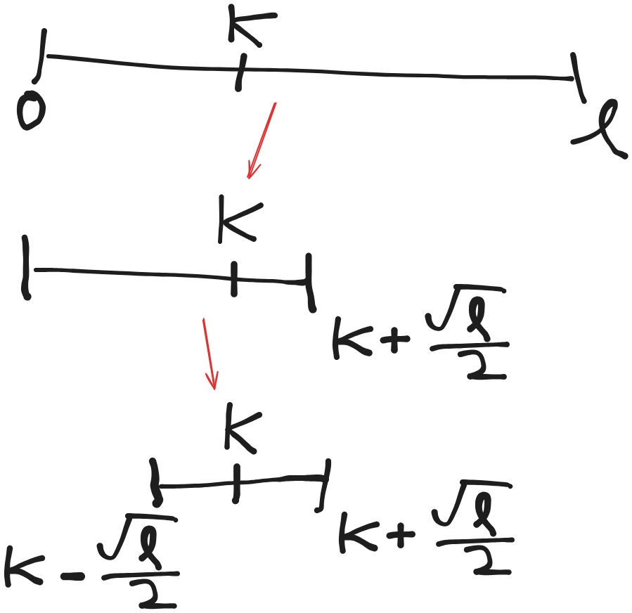
So the expected value of the square of $|K - k_i|$ is less than $\dfrac{l_i}{4}$, which means we should expect $|K - k_i| \leq \dfrac{\sqrt{l_i}}{2}$. So roughly speaking our guessed index should drop onto somewhere in $[K - \dfrac{\sqrt{l_i}}{2}, K + \dfrac{\sqrt{l_i}}{2}]$.

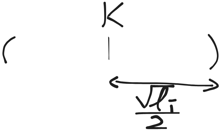
So each round we “chop” the array at one of the boundary of $[K - \dfrac{\sqrt{l_i}}{2}, K + \dfrac{\sqrt{l_i}}{2}]$. We could expect every 2 rounds the array shrinks from being with length $l_i$ to being with length $\sqrt{l_i}$.

That means our problem is broken down to a simlilar problem with size $\sqrt{l_i}$ and the process should ends when $\sqrt{l_i} \leq 2$ i.e. when you only got one choice of index to check in the next step. Some simple calculation tells us that when $i$ reaches $\log{\log{l}}$ the said condition will be true.

So the average case complexity should be $O(\log{\log{l}})$.

(Note that the reasoning above is very far away from being rigorous, it just helps us to guess the answer. I did not manage to prove it.)

The wheel we have reinvented

Well, turns out that the algorithm above is just interpolation search, nothing new.

Of cause since I did not manage to prove the time complexity which is the hardest part, I cannot claim any credits (more accurately, I cannot do so even if I figured out the proof). But I did find a proof by Y Perl². That proof was complex.

I just decided that things like this (and the previous blog post about reinventing the Catalan numbers) which rediscover established results by rethinking “101” topics should go into a series called something like “Wheels reinvention”.

As a sidenote, if we go the other way around and try to actively reverse engineering the discovery process of something we already knew, that will also be super fun… I should definitely try it.

More general cases?

Of cause, in real life no one would commit into a not-so-accurate guess and carry through it without a single change: throughout the process of checking the elements in the inferred positions, we gradually learn the actual distribution of the data and hence can adjust our expectation. For example, if you keep getting friends with name start with “L” when you try to find “Mike”, then probably your friend list skewed towards the first half of the alphabets (i.e. you got a lot of friends with names like “Angela”, “Bruce”, but less like “Pam”, “Veronica” etc.), especially those start with “L”. In this case we would like to adjust our assumption so that we put more “weights” to input starts with “L” - so from the current element (let’s say “Luigi”) we will skip more elements to look for “Mike”.

A typical flow of the process above would be:

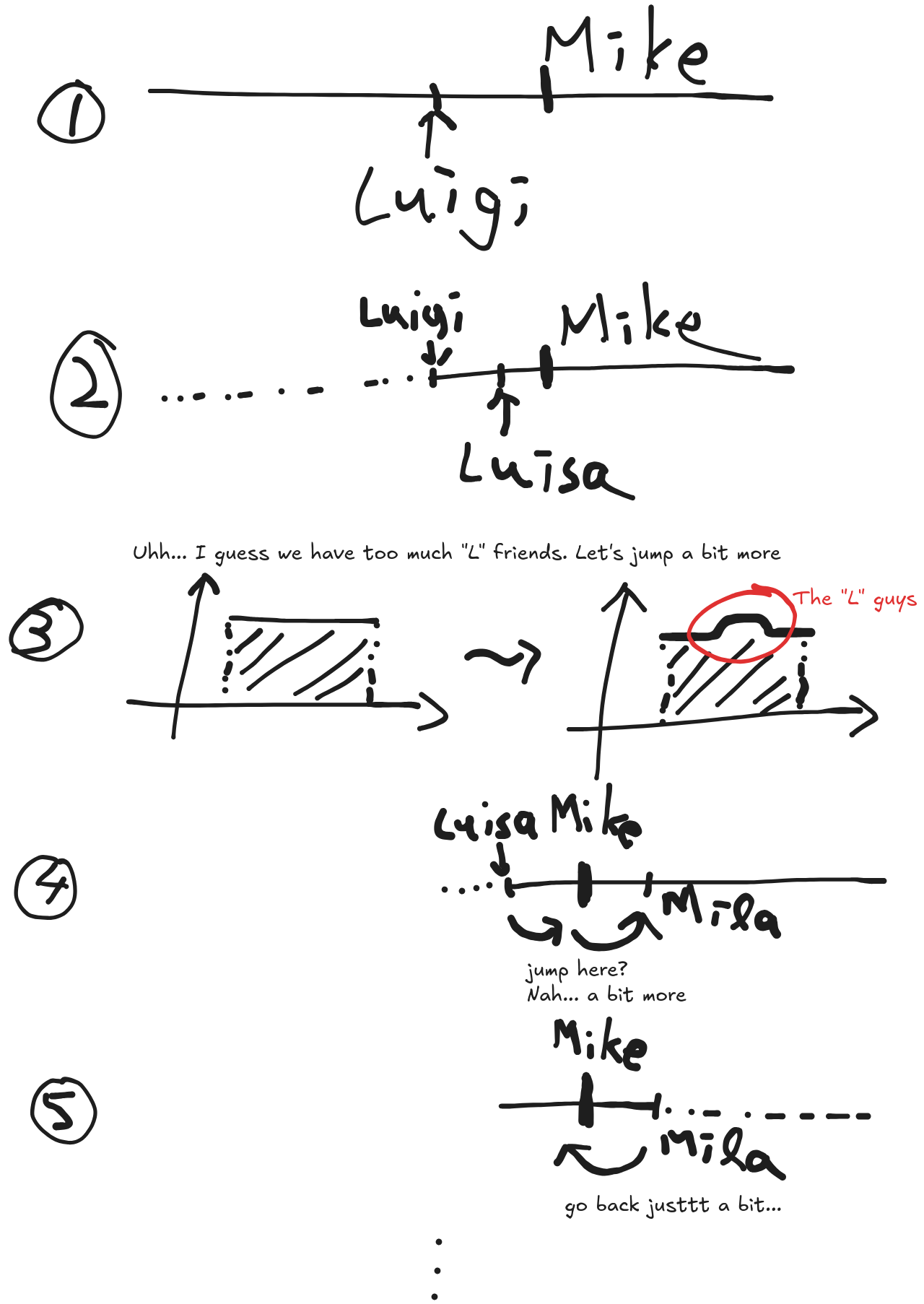
1. We assume all names are equally possible to appear in my contacts. The friend I want to look up is “Mike”, it is expected to be in the middle.
2. We check the middle, it is “Luigi”. So next we check the, let’s say $0.1^{th}$ position of the remaining array
3. We got “Luisa”.
4. Well I guess we have a lot of friends with names start with “L”. Maybe next we should check the $0.2^{th}$ position if the uniform distribution says it should be $0.1$ ? (I have to admit that I don’t know much people names start with “L” but after “Luisa”… but whatever)
5. We got “Mila”.
6. We’ve gone to far. If we assume uniform distribution we should check $0.9$. But remember there are a lot of “L” friends, so it should be like $0.95$.
7. and so on…

Things go a bit hand wavy at this point. Rigorously defining this generalized algorithm and analyzing it will likely take good effort.